
Visualization with `ggplot2`
Adam J Sullivan
Assistant Professor of Biostatistics
Brown University
ggplot2
Appropriate graphical analysis may make the conclusions so clearcut that detailed specific analysis is unnecessary
-- David Cox (1978)
ggplot2
- We will begin our journey into statistical graphics with the package
ggplot2. - This is a package by Hadley Wickham and is part of the tidyverse.
- It is a very comprehensive and easily adaptable language of graphics.
What can't ggplot2 do?
- A good place to start might be with what
ggplot2cannot do:- 3d graphs.
- Interactive graphs, use
ggvis - DAGs, see
igraph
- We will now focus on all the things it can do.
ggplot2 components
ggplot2is built off the grammar of graphics with a very intuitive structure.- The base graphics built into R require the use of many different functions and each of them seem to have their own method for how to use them.
ggplot2will be more fluid and the more you learn about it the more amazing of graphics you can create.
ggplot2 components
- We will get started with the components of every
ggplot2object:- data
- aesthetic mappings between variables in the data and visual properties.
- At least one layer which describes how to render the data.
- Many of these are with the
geom_foo()function.
Our Data
- We will be working with data from fivethirtyeight
- We can access this by installing the package in R:
install.packages("fivethiryeight")
library(fivethirtyeight)
Our Data
- We will work with data from the article: Comic Books Are Still Made By Men, For Men And About Men
- We can access this data by calling the following:
comic_characters
Comic Characters Data
## # A tibble: 23,272 x 16
##    publisher page_id name  urlslug id    align eye   hair  sex   gsm
##    <chr>       <int> <chr> <chr>   <chr> <ord> <chr> <chr> <chr> <chr>
##  1 Marvel       1678 Spid~ "\\/Sp~ Secr~ Good~ Haze~ Brow~ Male~ <NA>
##  2 Marvel       7139 Capt~ "\\/Ca~ Publ~ Good~ Blue~ Whit~ Male~ <NA>
##  3 Marvel      64786 "Wol~ "\\/Wo~ Publ~ <NA>  Blue~ Blac~ Male~ <NA>
##  4 Marvel       1868 "Iro~ "\\/Ir~ Publ~ Good~ Blue~ Blac~ Male~ <NA>
##  5 Marvel       2460 Thor~ "\\/Th~ No D~ Good~ Blue~ Blon~ Male~ <NA>
##  6 Marvel       2458 Benj~ "\\/Be~ Publ~ Good~ Blue~ No H~ Male~ <NA>
##  7 Marvel       2166 Reed~ "\\/Re~ Publ~ Good~ Brow~ Brow~ Male~ <NA>
##  8 Marvel       1833 Hulk~ "\\/Hu~ Publ~ Good~ Brow~ Brow~ Male~ <NA>
##  9 Marvel      29481 Scot~ "\\/Sc~ Publ~ <NA>  Brow~ Brow~ Male~ <NA>
## 10 Marvel       1837 Jona~ "\\/Jo~ Publ~ Good~ Blue~ Blon~ Male~ <NA>
## # ... with 23,262 more rows, and 6 more variables: alive <chr>,
## #   appearances <int>, first_appearance <chr>, month <chr>, year <int>,
## #   date <date>
Comic Characters Data
- We can see the names of the variables by using the
names()function:
names(comic_characters)
##  [1] "publisher"        "page_id"          "name"
##  [4] "urlslug"          "id"               "align"
##  [7] "eye"              "hair"             "sex"
## [10] "gsm"              "alive"            "appearances"
## [13] "first_appearance" "month"            "year"
## [16] "date"
ggplot() Basics
- We will begin with a basic graph of appearances by alignment
library(ggplot2)
ggplot(data=comic_characters, aes(x=align, y=appearances))
ggplot() Basics
ggplot() Statement
- We can see that all we have is the basic layout of axis.
- The data and aes gives us the basic layout.
- We need
geom_foo()to make a proper graph.
geom_point() Statement
- We can add
geom_point()to this:
ggplot(data=comic_characters, aes(x=align, y=appearances)) +
  geom_point()
geom_point() Statement
Other graphs
- This graph is not the best use for out data.
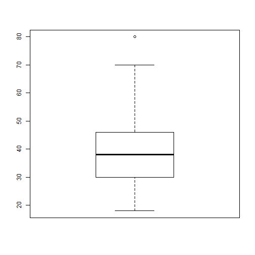
- We could try boxplots instead:
ggplot(data=comic_characters, aes(x=align, y=appearances)) +
  geom_boxplot()
Other graphs
Quick Transformation
- We may be having a hard time seeing this due to the outliers in the data.
- We can try a log transform.
- The code below will do this
- By the end of today you will understand this code
comic_characters <- comic_characters %>%
  mutate(log_app = log(appearances))
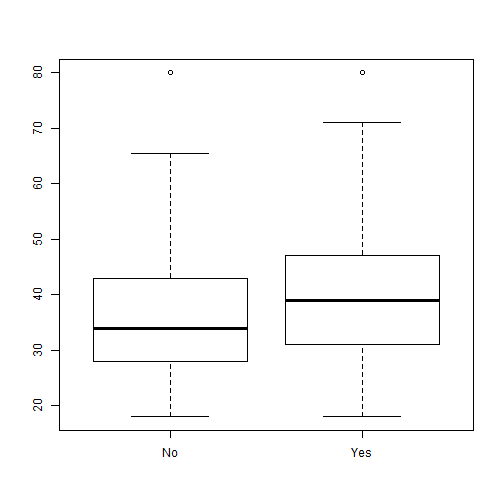
Boxplots Again
Bar Graphs
- We could then consider simple bar graphs
- For example if we wanted to know how many characters of each type there were:
ggplot(data=comic_characters, aes(x=align)) +
  geom_bar()
- Note: With bar graphs we only need the x-axis.
Bar Graphs
Basic Template
ggplot(data= <DATA>, aes(x=<X-VARIABLE>, y=<Y-VARIABLE>)) +
    <GEOM_FUNCTION>()
Aesthetics
Aesthetics
- The basic aesthetics are mapping the data to the x and y axis.
- We can also add:
alpha: makes points transparent to see overlaps betterfill: Fills objects with colorcolor: Changes color of points or lines.shape: Changes spape of points
Aesthetics: alpha
ggplot(data=comic_characters, aes(x=align, y=log_app)) +
  geom_point(aes(alpha=1/100))
Aesthetics: alpha
Aesthetics: alpha
- It can be hard to see the transparency when they are so close.
- We can set the transparency to a variable
YOUR TURN
- Set
alpha=year - How does this change things?
Aesthetics: alpha
Aesthetics: color
- We can easily change the color of points and lines using
color
ggplot(data=comic_characters, aes(x=align, y=log_app)) +
  geom_point(aes(color=publisher))
Aesthetics: color
YOUR TURN
- Set
color="blue" - How does this change things?
Aesthetics: shapes
- We can change the shape of points based on different variables.
ggplot(data=comic_characters, aes(x=align, y=log_app)) +
  geom_point(aes(shape=publisher))
Aesthetics: shapes
Your Turn
- Try using both shape and color.
- How does this add dimensionality to the graph?
Aesthetics: fill
- We can fill objects with color as well
ggplot(data=comic_characters, aes(x=align)) +
  geom_bar(aes(fill="blue"))
Aesthetics: fill
- This doesnt have the same effect as
color
Aesthetics: fill
- We can use other variables to add dimensionality
ggplot(data=comic_characters, aes(x=align)) +
  geom_bar(aes(fill=publisher))
Aesthetics: fill
Geoms
Geoms
- There are many
geom_foo()functions we can use. - The Cheatsheet on
ggplot()is a good place to start for more.
Other Plots: Density
Other Plots: Density
Other Plots: Histogram
Piping or Chaining Data
Piping or Chaining
- We will discuss a concept that will help us greatly when it comes to working with our data.
- The usual way to perform multiple operations in one line is by nesting.
Piping or Chaining
To consider an example we will look at the data provided in the gapminder package:
library(gapminder)
head(gapminder)
## # A tibble: 6 x 6
##   country     continent  year lifeExp      pop gdpPercap
##   <fct>       <fct>     <int>   <dbl>    <int>     <dbl>
## 1 Afghanistan Asia       1952    28.8  8425333      779.
## 2 Afghanistan Asia       1957    30.3  9240934      821.
## 3 Afghanistan Asia       1962    32.0 10267083      853.
## 4 Afghanistan Asia       1967    34.0 11537966      836.
## 5 Afghanistan Asia       1972    36.1 13079460      740.
## 6 Afghanistan Asia       1977    38.4 14880372      786.
Nesting vs Chaining
- Let's say that we want to have the GDP per capita and life expectancy Kenya.
- Traditionally speaking we could do this in a nested manner:
filter(select(gapminder, country, lifeExp, gdpPercap), country=="Kenya")
Nesting vs Chaining
- It is not easy to see exactly what this code was doing but we can write this in a manner that follows our logic much better.
- The code below represents how to do this with chaining.
gapminder %>%
    select(country, lifeExp, gdpPercap) %>%
    filter(country=="Kenya")
Breaking Down the Code
- We now have something that is much clearer to read.
- Here is what our chaining command says:
- Take the
gapminderdata - Select the variables:
country,lifeExpandgdpPercap. - Only keep information from Kenya.
- Take the
- The nested code says the same thing but it is hard to see what is going on if you have not been coding for very long.
Breaking Down the Code
- The result of this search is below:
# A tibble: 12 x 3
   country lifeExp gdpPercap
    <fctr>   <dbl>     <dbl>
 1   Kenya  42.270  853.5409
 2   Kenya  44.686  944.4383
 3   Kenya  47.949  896.9664
 4   Kenya  50.654 1056.7365
 5   Kenya  53.559 1222.3600
 6   Kenya  56.155 1267.6132
 7   Kenya  58.766 1348.2258
 8   Kenya  59.339 1361.9369
 9   Kenya  59.285 1341.9217
10   Kenya  54.407 1360.4850
11   Kenya  50.992 1287.5147
12   Kenya  54.110 1463.2493
What is %>%
- In the previous code we saw that we used
%>%in the command you can think of this as saying then. - For example:
gapminder %>%
    select(country, lifeExp, gdpPercap) %>%
    filter(country=="Kenya")
What Does this Mean?
- This translates to:
- Take Gapminder then select these columns select(country, lifeExp, gdpPercap) then filter out so we only keep Kenya
Why Chain?
- We still might ask why we would want to do this.
- Chaining increases readability significantly when there are many commands.
- With many packages we can replace the need to perform nested arguments.
- The chaining operator is automatically imported from the magrittr package.
User Defined Function
- Let's say that we wish to find the Euclidean distance between two vectors say,
x1andx2. - We could use the math formula:
\[\sqrt{\sum(x_1-x_2)^2}\]
User Defined Function
- In the nested manner this would be:
x1 <- 1:5; x2 <- 2:6
sqrt(sum((x1-x2)^2))
User Defined Function
- However, if we chain this we can see how we would perform this mathematically.
# chaining method
(x1-x2)^2 %>% sum() %>% sqrt()
- If we did it by hand we would perform elementwise subtraction of
x2fromx1then we would sum those elementwise values then we would take the square root of the sum.
User Defined Function
# chaining method
(x1-x2)^2 %>% sum() %>% sqrt()
## [1] 2.236068
- Many of us have been performing calculations by this type of method for years, so that chaining really is more natural for us.