
Regression Basics Part 2
Adam J Sullivan
Assistant Professor of Biostatistics
Brown University
One Continuous
One Continuous Covariate
- We will consider one continuous covariate.
- We will consider year.
Example: Year and Appearances
- Consider the effect of year on appearances.
- With categorical data we plotted this with box-whisker plots.
- We can now use a scatter plot
Scatter Plot: Year and Appearances
ggplot(comic_characters, aes(year, appearances)) +
  geom_point() +
  geom_smooth(method="lm") +
  xlab("Year") +
  ylab("Appearances")
Scatter Plot: Year and Appearances
Modeling What We See
- There might not be a connection or there might be a very small one, let's explore further.
- How can we do this?
- How does linear regression work?
How do we Quantify this?
- One way we could quantify this is \[\mu_{y|x} = \beta_0 + \beta_1X\]
- where
- \(\mu_{y|x}\) is the mean time for those whose year is \(x\).
- \(\beta_0\) is the \(y\)-intercept (mean value of \(y\) when \(x=0\), \(\mu_y|0\))
- \(\beta_1\) is the slope (change in mean value of \(Y\) corresponding to 1 unit increase in \(x\)).
Population Regression Line
- With the population regression line we have that the distribution of appearances for those at a particular year, \(x\), is approximately normal with mean, \(\mu_{y|x}\), and standard deviation, \(\sigma_{y|x}\).
Population Regression Line
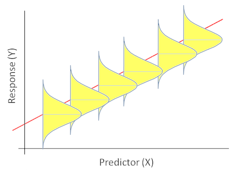
Population Regression Line
- This shows the scatter about the mean due to natural variation. To accommodate this scatter we fit a regression model with 2 parts:
- Systematic Part
- Random Part
The Model
- This leads to the model \[Y = \beta_0 + \beta_1X + \varepsilon\]
- Where \(\beta_0+\beta_1X\) is the systematic part of the model and implies that \[E(Y|X=x) = \mu_{y|x} = \beta_0 + \beta_1x\]
- the variation part where we have \(\varepsilon\sim N(0,\sigma^2)\) which is independent of \(X\).
What do We Have?
- Consider the scenario where we have \(n\) subjects and for each subject we have the data points \((x,y)\).
- This leads to us having data in the form \((X_i,Y_i)\) for \(i=1,\ldots,n\).
- Then we have the model: \[Y_i = \beta_0 + \beta_1X_i + \varepsilon_i\]
- \(Y_i|X_i \sim N\left(\beta_0 + \beta_1X_i , \sigma^2\right)\)
- \(E(Y_i|X_i) = \mu_{y|x} = \beta_0 + \beta_1X_i\)
- \(Var(Y|X_i ) = \sigma^2\)
Picture of this
What Does This Tell Us?
- We can refer back to our scatter plot now and discuss what is the "best" line.
- Given the previous image we can see that a good estimator would somehow have smaller residual errors.
- So the "best" line would minimize the errors.
Residual Errors

In Comes Least Squares
- The least squares estimator of regression coefficients in the estimator that minimizes the sum of squared errors.
- We denote these estimators as \(\hat{\beta}_0\) and \(\hat{\beta}_1\).
- In other words we attempt to minimize \[\sum_{i=1}^n \left(\varepsilon_i\right)^2 = \sum_{i=1}^n \left(Y_i - \hat{\beta}_0 - \hat{\beta}_1X_i\right)^2\]
Inferences on OLS
- Once we have our intercept and slope estimators the next step is to determine if they are significant or not.
- Typically with hypothesis testing we have needed the following:
- Population/Assumed Value of interest
- Estimated value
- Standard error of Estimate
Confidence Interval Creation
- with 95% confidence intervals of \[\hat{\beta}_1 \pm t_{n-2, 0.975} \cdot se\left(\hat{\beta}_1\right)\] \[\hat{\beta}_0 \pm t_{n-2, 0.975} \cdot se\left(\hat{\beta}_0\right)\]
- In general we can find a \(100(1-\alpha)\%\) confidence interval as \[\hat{\beta}_1 \pm t_{n-2, 1-\dfrac{\alpha}{2}} \cdot se\left(\hat{\beta}_1\right)\] \[\hat{\beta}_0 \pm t_{n-2, 1-\dfrac{\alpha}{2}} \cdot se\left(\hat{\beta}_0\right)\]
Example: Year and Appearances
model <- lm(appearances~year, data=comic_characters)
tidy(model, conf.int=TRUE)[,-c(3:4)]
glance(model)
Example: Year and Appearances
## # A tibble: 1 x 11
##   r.squared adj.r.squared sigma statistic  p.value    df  logLik    AIC
##       <dbl>         <dbl> <dbl>     <dbl>    <dbl> <int>   <dbl>  <dbl>
## 1    0.0146        0.0145  93.8      313. 1.74e-69     2 -1.26e5 2.52e5
## # ... with 3 more variables: BIC <dbl>, deviance <dbl>, df.residual <int>
Interpreting the Coefficients: Continuous
- Before we can discuss the regression coefficients we need to understand how to interpret what these coefficients mean.
- \(\beta_0\) is mean value for \(Y\) when \(X=0\).
- What about \(\beta_1\)?
Interpreting the Coefficients: Continuous
- Then we consider \(\beta_1\) to see the meaning of this we do the following \[ \begin{aligned} E(Y|X=x+1) - E(Y|X=x) &= \beta_0 + \beta_1(x+1) - \beta_0 - \beta_1x\\ &= \beta_1 \end{aligned} \]
Interpreting the Coefficients: Continuous
- We consider \(\beta_0\) first.
- Does this value have meaning with our current data?
- The estimated value of time level is only applicable to year within the range of our data.
- Many times the intercept is scientifically meaningless.
- Even if meaningless on its own, \(\beta_0\) is necessary to specify the equation of our regression line.
- Note: People do sometimes use mean centered data and the intercept is then interpretable.
Interpreting the Coefficients: Continuous
- This gives us the interpretation that \(\beta_1\) represents the mean change in outcome \(Y\) given a one unit increase in predictor \(X\).
- This is not an actual prescription though, this is considering different subjects or groups of subjects who differ by one unit.
- Below are correct interpretations of \(\beta_1\) in our example.
- These results display that the mean difference in appearances for a 1 year difference is -0.596
- These results display that the mean difference in time for a 10 year difference is -5.96
Multiple Regression
- We have been discussing simple models so far.
- This works well when you have:
- Randomized Data to test between specific groups (Treatment vs Control)
- In most situations we need look at more than just one relationship.
- Think of this as needing more information to tell the entire story.
Multiple Linear Regression with appearances
- First start with univariate models
- Then perform the multiple model
Multivariate Models
mod3 <- lm(appearances~publisher + year, data=comic_characters)
tidy3 <- tidy(mod3, conf.int=T)[,-c(3:4)]
tidy3
## # A tibble: 3 x 5
##   term             estimate  p.value  conf.low conf.high
##   <chr>               <dbl>    <dbl>     <dbl>     <dbl>
## 1 (Intercept)      1265.    9.81e-78  1133.     1398.
## 2 publisherMarvel    -9.54  1.24e-11   -12.3      -6.78
## 3 year               -0.624 5.93e-75    -0.690    -0.557
Interpreting Multiple Coefficients
- The intercept is when all coefficients are zero.
- Each other coefficient is interpreted in context to another.
Interpreting Multiple Coefficients: Our Example
- Intercept: DC average appearances at year 0. Not Meaningful
- Publisher Coefficient: If we consider 2 characters in the same year, the character from Marvel will have on average 9.54 less appearances than the character from DC.
- Year Coefficient: If we consider 2 characters from the same publisher, an increase in 1 year will lead to on average 0.62 less appearances.
Multiple Regression
Multiple Regression
- We have been discussing simple models so far.
- This works well when you have:
- Randomized Data to test between specific groups (Treatment vs Control)
- In most situations we need look at more than just one relationship.
- Think of this as needing more information to tell the entire story.
Motivating Example
- Health disparities are very real and exist across individuals and populations.
- Before developing methods of remedying these disparities we need to be able to identify where there are disparities.In this homework we will consider a study by (Asch & Armstrong, 2007).
- This paper considers 222 patients with localized prostate cancer.
Motivating Example
- The table below partitions patients by race, hospital and whether or not the patient received a prostatectomy.
| Race | Prostatectomy | No Prostatectomy | |
|---|---|---|---|
| University Hospital | White | 54 | 37 |
| Black | 7 | 5 | |
| VA Hospital | White | 11 | 29 |
| Black | 22 | 57 |
Loading the Data
You can load this data into R with the code below:
phil_disp <- read.table("https://drive.google.com/uc?export=download&id=0B8CsRLdwqzbzOXlIRl9VcjNJRFU", header=TRUE, sep=",")
The Data
This dataset contains the following variables:
| Variable | Description |
|---|---|
| hospital | 0 - University Hospital |
| 1 - VA Hospital | |
| race | 0 - White |
| 1 - Black | |
| surgery | 0 - No prostatectomy |
| 1 - Had Prostatectomy | |
| number | Count of people in Category |
Consider Prostatectomy by Race
library(broom)
prost_race <- glm(surgery ~ race, weight=number, data= phil_disp,
                  family="binomial")
tidy(prost_race, exponentiate=T, conf.int=T)[,-c(3:4)]
## # A tibble: 2 x 5
##   term        estimate p.value conf.low conf.high
##   <chr>          <dbl>   <dbl>    <dbl>     <dbl>
## 1 (Intercept)    0.985 0.930      0.699     1.39
## 2 race           0.475 0.00895    0.269     0.825
Consider Prostatectomy by Race
- What can we conclude?
- What kind of policy might we want to invoke based on this discovery?
Consider Prostatectomy by Hospital
prost_hosp <- glm(surgery ~ hospital, weight=number, data= phil_disp,
                  family="binomial")
tidy(prost_hosp, exponentiate =T, conf.int=T)[,-c(3:4)]
## # A tibble: 2 x 5
##   term        estimate    p.value conf.low conf.high
##   <chr>          <dbl>      <dbl>    <dbl>     <dbl>
## 1 (Intercept)    1.45  0.0627        0.984     2.16
## 2 hospital       0.264 0.00000341    0.149     0.460
Consider Prostatectomy by Hospital
- What can we conclude?
Multiple Regression of Prostatectomy
prost <- glm(surgery ~ hospital + race, weight=number, data= phil_disp,
             family="binomial")
tidy(prost, exponentiate=T, conf.int=T)[,-c(3:4)]
## # A tibble: 3 x 5
##   term        estimate  p.value conf.low conf.high
##   <chr>          <dbl>    <dbl>    <dbl>     <dbl>
## 1 (Intercept)    1.45  0.0682      0.976     2.18
## 2 hospital       0.264 0.000124    0.131     0.515
## 3 race           0.998 0.996       0.501     2.04
Multiple Regression of Prostatectomy
- What can We conclude?
- What happened here?
- Does this change our policy suggestion from before?
Benefits of Multiple Regression
- Multiple Regression helps us tell a more complete story.
- Multiple regression controls for confounding.
Confounding
- Associated with both the Exposure and the Outcome
- Even if the Exposure and Outcome are not related, unmeasured confounding can show that they are.
What Do We Do with Confounding?
- We must add all confounders into our model.
- Without adjusting for confounders are results may be highly biased.
- Without adjusting for confounding we may make incorrect policies that do not fix the problem.
Multiple Linear Regression with appearances
- First start with univariate models
- Then perform the multiple model
Multivariate Models
library(broom)
library(fivethirtyeight)
mod3 <- lm(appearances~publisher + year, data=comic_characters)
tidy3 <- tidy(mod3, conf.int=T)[,-c(3:4)]
tidy3
## # A tibble: 3 x 5
##   term             estimate  p.value  conf.low conf.high
##   <chr>               <dbl>    <dbl>     <dbl>     <dbl>
## 1 (Intercept)      1265.    9.81e-78  1133.     1398.
## 2 publisherMarvel    -9.54  1.24e-11   -12.3      -6.78
## 3 year               -0.624 5.93e-75    -0.690    -0.557
Interpreting Multiple Coefficients
- The intercept is when all coefficients are zero.
- Each other coefficient is interpreted in context to another.
Interpreting Multiple Coefficients: Our Example
- Intercept: DC average appearances at year 0. Not Meaningful
- Publisher Coefficient: If we consider 2 characters in the same year, the character from Marvel will have on average 9.54 less appearances than the character from DC.
- Year Coefficient: If we consider 2 characters from the same publisher, an increase in 1 year will lead to on average 0.62 less appearances.
Further Example: Bike Sharing Data
- We have hourly data spanning 2 years
- This dataset has the first 19 days of each month.
- Goal is to find the total count of bike rented.
Further Example: Bike Sharing Data
| Data | Fields |
|---|---|
| datetime | hourly date + timestamp |
| season | 1 = spring, 2 = summer, 3 = fall, 4 = winter |
| holiday | whether the day is considered a holiday |
| workingday | whether the day is neither a weekend nor holiday |
Further Example: Bike Sharing Data
| Data | Fields |
|---|---|
| weather | 1: Clear, Few clouds, Partly cloudy, Partly cloudy |
| 2: Mist + Cloudy, Mist + Broken clouds, Mist + Few clouds, Mist | |
| 3: Light Snow, Light Rain + Thunderstorm + Scattered clouds, Light Rain + Scattered clouds | |
| 4: Heavy Rain + Ice Pallets + Thunderstorm + Mist, Snow + Fog | |
| temp | temperature in Celsius |
Further Example: Bike Sharing Data
| Data | Fields |
|---|---|
| atemp | "feels like" temperature in Celsius |
| humidity | relative humidity |
| windspeed | wind speed |
| casual | number of non-registered user rentals initiated |
| registered | number of registered user rentals initiated |
| count | number of total rentals |
Univariate Regressions
library(readr)
library(tidyverse)
bikes <- read_csv("../Notes/Data/bike_sharing.csv") %>%
        mutate(season = as.factor(season)) %>%
        mutate(weather=as.factor(weather))
Univariate Regressions
mod1 <- lm(count~season, data=bikes)
mod2 <- lm(count~holiday, data=bikes)
mod3 <- lm(count~workingday, data=bikes)
mod4 <- lm(count~weather, data=bikes)
mod5 <- lm(count~temp, data=bikes)
mod6 <- lm(count~atemp, data=bikes)
mod7 <- lm(count~humidity, data=bikes)
mod8 <- lm(count~windspeed, data=bikes)
mod9 <- lm(count~casual, data=bikes)
mod10 <- lm(count~registered, data=bikes)
Univariate Regressions
library(broom)
tidy1 <- tidy( mod1, conf.int=T )[-1, -c(3:4) ]
tidy2 <- tidy(mod2, conf.int=T )[-1, -c(3:4) ]
tidy3 <- tidy(mod3 , conf.int=T)[-1, -c(3:4) ]
tidy4 <- tidy(mod4 , conf.int=T)[-1, -c(3:4) ]
tidy5 <- tidy(mod5, conf.int=T)[-1, -c(3:4) ]
tidy6 <- tidy(mod6 , conf.int=T)[-1, -c(3:4) ]
tidy7 <- tidy(mod7 , conf.int=T)[-1, -c(3:4) ]
tidy8 <- tidy(mod8 , conf.int=T)[-1, -c(3:4) ]
tidy9 <- tidy(mod9, conf.int=T)[-1, -c(3:4) ]
tidy10 <- tidy(mod10, conf.int=T)[-1, -c(3:4) ]
bind_rows(tidy1, tidy2, tidy3, tidy4, tidy5, tidy6, tidy7, tidy8, tidy9, tidy10)
Univariate Regressions
## # A tibble: 14 x 5
##    term       estimate   p.value conf.low conf.high
##    <chr>         <dbl>     <dbl>    <dbl>     <dbl>
##  1 season2       98.9  9.76e- 94    89.6     108.
##  2 season3      118.   1.06e-131   109.      127.
##  3 season4       82.6  2.13e- 66    73.3      92.0
##  4 holiday       -5.86 5.74e-  1   -26.3      14.6
##  5 workingday     4.51 2.26e-  1    -2.80     11.8
##  6 weather2     -26.3  4.32e- 11   -34.1     -18.5
##  7 weather3     -86.4  3.29e- 40   -99.1     -73.7
##  8 weather4     -41.2  8.18e-  1  -393.      311.
##  9 temp           9.17 0.            8.77      9.57
## 10 atemp          8.33 0.            7.96      8.70
## 11 humidity      -2.99 2.92e-253    -3.15     -2.82
## 12 windspeed      2.25 2.90e- 26     1.83      2.66
## 13 casual         2.50 0.            2.45      2.55
## 14 registered     1.16 0.            1.16      1.17
Multivariate
mod.final <- lm(count~season+weather+humidity+windspeed, data=bikes)
tidy(mod.final)[-1,-c(3:4)]
glance(mod.final)
Multivariate
## # A tibble: 8 x 3
##   term      estimate   p.value
##   <chr>        <dbl>     <dbl>
## 1 season2    116.    1.40e-145
## 2 season3    148.    7.52e-227
## 3 season4    118.    1.74e-147
## 4 weather2    20.0   1.38e-  7
## 5 weather3     0.124 9.84e-  1
## 6 weather4   162.    3.19e-  1
## 7 humidity    -3.49  3.86e-273
## 8 windspeed    0.633 2.05e-  3
Multivariate
## # A tibble: 1 x 11
##   r.squared adj.r.squared sigma statistic p.value    df  logLik    AIC
##       <dbl>         <dbl> <dbl>     <dbl>   <dbl> <int>   <dbl>  <dbl>
## 1     0.195         0.194  163.      329.       0     9 -70865. 1.42e5
## # ... with 3 more variables: BIC <dbl>, deviance <dbl>, df.residual <int>