
Non-Parametric Survival Analysis
Adam J Sullivan
Assistant Professor of Biostatistics
Brown University
Estimation of a Survival Curves
Estimation of a Survival Curves
Many times we use nonparametric estimators - This requires that \(C\) is independent of \(T\).
- Kaplan-Meier estimate of \(S(t)\)
- Confidence intervals for \(S(t)\)
- Nelson-Aalen estimate for \(\Lambda(t)\)
- Confidence intervals for \(\Lambda(t)\)
Example: No Censoring
We begin with an example of Remission times (time to relapse) measured in weeks for 21 leukemia patients: \[T_i = 1,1,2,2,3,4,4,5,5,8,8,8,8,11,11,12,12,15,17,22,23\]
- Not there are no censored observations here
- When there is no censoring (all subjects experience the event), fix a time \(t\) and consider the indicator variable \[I(T\ge t)\] This is a binomial random variable with \[\Pr\left(I(T\ge t)=1\right)= S(t)\]
Example: No Censoring
Our goal is to estimate \(S(t)\) so we consider:
\[\hat{S}(t) = \dfrac{1}{n}\sum_{i=1}^n I(T_i\ge t)\]
For example we have that
- \(\hat{S}(10) = \dfrac{8}{10}\)
- \(\hat{S}(19) = \dfrac{8}{10}\)
Example: No Censoring
Then since this is a binomial random variable, we can consider the variance of \(S(t)\) as \[Var\left[S(t)\right]= nS(t)\left[1-S(t)\right]\]
library(survival)
T.1 <- c(1,1,2,2,3,4,4,5,5,8,8,8,8,11,11,12,12,15,17,22,23)
event.1 <- rep(1, length(T.1))

Y <- Surv(T.1, event.1==1)
K.M <- survfit(Y~1)
summary(K.M)
Example: No Censoring
## Call: survfit(formula = Y ~ 1)
##
##  time n.risk n.event survival std.err lower 95% CI upper 95% CI
##     1     21       2   0.9048  0.0641      0.78754        1.000
##     2     19       2   0.8095  0.0857      0.65785        0.996
##     3     17       1   0.7619  0.0929      0.59988        0.968
##     4     16       2   0.6667  0.1029      0.49268        0.902
##     5     14       2   0.5714  0.1080      0.39455        0.828
##     8     12       4   0.3810  0.1060      0.22085        0.657
##    11      8       2   0.2857  0.0986      0.14529        0.562
##    12      6       2   0.1905  0.0857      0.07887        0.460
##    15      4       1   0.1429  0.0764      0.05011        0.407
##    17      3       1   0.0952  0.0641      0.02549        0.356
##    22      2       1   0.0476  0.0465      0.00703        0.322
##    23      1       1   0.0000     NaN           NA           NA
Example: No Censoring
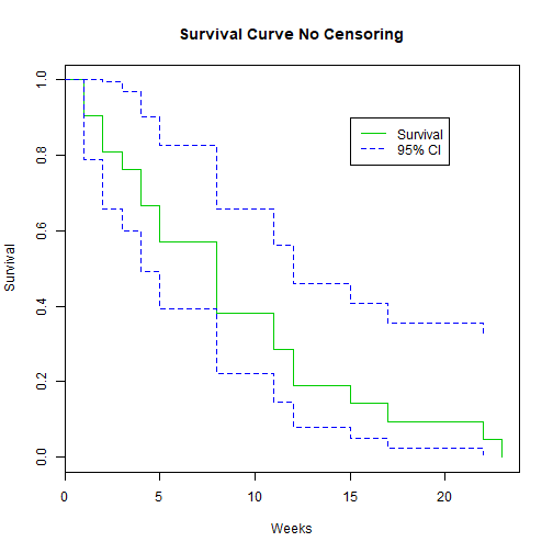
library(GGally)
plot(K.M, main="Survival Curve No Censoring", xlab="Weeks", ylab="Survival", col=c(3,4, 4))
legend(15, .9, c("Survival", "95% CI"), lty = 1:2, col=c(3,4))
Example: No Censoring
Example: No Censoring
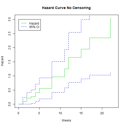
We can also plot the hazard:
library(GGally)
plot(K.M, fun="cumhaz", main="Hazard Curve No Censoring", xlab="Weeks", ylab="Hazard", col=c(3,4, 4))
legend(0, 3, c("Hazard", "95% CI"), lty = 1:2, col=c(3,4))
Example: No Censoring
We can also plot the hazard:
Example: Censoring
We go back to the same study as before. This was published in 1965 by Gehan. There were 21 patients in a control group and 21 patients in a drug group. They were followed to see how long in weeks before they relapsed.
- Drug: 6+, 6, 6, 6, 7, 9+, 10+, 10, 11+, 13, 16, 17+, 19+, 20+, 22, 23, 25+, 32+, 32+, 34+, 35+
- Control: 1, 1, 2, 2, 3, 4, 4, 5, 5, 8, 8, 8, 8, 11, 11, 12, 12, 15, 17, 22, 23
We can enter these into R but this time we need to account for the censoring
Example: Censoring
T.1 <- c(1,1,2,2,3,4,4,5,5,8,8,8,8,11,11,12,12,15,17,22,23)
event.1 <- rep(1, length(T.1))
group.1 <- rep(0,length(T.1))

T.2 <- c(6,6,6,6,7,9,10,10,11,13,16,17,19,20,22,23,25,32,32,34,35)
event.2 <- c(0,1,1,1,1,0,0,1,0,1,1,0,0,0,1,1,0,0,0,0,0)
group.2 <- rep(1, length(T.2))

T.all <- c(T.1,T.2)
event.all <- c(event.1,event.2)
group.all <- c(group.1, group.2)

leuk2 <- data.frame(cbind(T.all, event.all, group.all))
Kaplan-Meier Estimator
The control group was easy to analyze as it had no censoring so we could calculate it by hand. However with the introduction to censoring we need a new estimator.
- Kaplan-Meier is a non-parametric method.
- No assumptions of distribution
- We define patients to be at risk at time \(t\) if they have not experienced the event just before time \(t\) and are not yet censored just before time \(t\).
Product Limit Method
Let
- \(t_i=\) distinct observed failure times (uncensored), in increasing order such that \(t_1
- \(K=\) number of distinct failure times
- \(n_i=\) number of subjects at risk at \(t_i\)
- \(d_i=\) number of failures at even \(t_i\)
- \(\hat{p}_i=\dfrac{d_i}{n_i}=\) estimated risk of failure at \(t_i\) given at risk at \(t_i\).
- \(\hat{q}_i= 1-\hat{p}_i=\) estimated proportion surviving \(t_i\) given at risk at \(t_i\).
Kaplan-Meier
The Kaplan-Meier estimate of survival is:
- \(\hat{S}(0)=1\)
- It drops after each of the distinct failure times.
- Let \(t_k\) be the \(k^{\text{th}}\) observed event time.
- In order to have \(T_i>t_k\), subject \(i\) needs to
- be at risk at \(t_1\) and have \(T_i>t_1\) and
- be at risk at \(t_2\) and have \(T_i>t_2\) and
- \(\qquad\qquad\vdots\)
- be at risk at \(t_k\) and have \(T_i>t_k\).
- In order to have \(T_i>t_k\), subject \(i\) needs to
Kaplan Meier
Then
\[\Pr(T_i>t_k) = \Pr(T_i>t_1|\text{at risk at }t_1) \times \cdots \times \Pr(T_i>t_k|\text{at risk at }t_k)\]
Then we have that for \(0\le t < t_1\)
\[\hat{S}(t) = 1 \]
Kaplan Meier
Then for \(t_1 \le t < t_2\) we have that:
\[\begin{aligned} \hat{S}(t) &= \Pr(T>t_1)|\text{at risk at }t_1)\\ &= 1- \dfrac{d_1}{n_1}\\ &= \dfrac{n_1-d_1}{n_1}\\ \end{aligned}\]
Kaplan Meier
for \(t_2 \le t < t_3\) we have that:
\[\begin{aligned} \hat{S}(t) &= \Pr(T>t_1)|\text{at risk at }t_1) \times \Pr(T>t_2)|\text{at risk at }t_2)\\ &= \hat{q}_1 \times \hat{q}_2\\ &= \left(\dfrac{n_1-d_1}{n_1}\right)\left(\dfrac{n_2-d_2}{n_2}\right)\\ &= \prod_{j=1}^2 \left(\dfrac{n_j-d_j}{n_j}\right) \end{aligned}\]
Kaplan Meier
thus for any \(t_i \[\hat{S}(t) = \prod_{j=1}^i \left(\dfrac{n_j-d_j}{n_j}\right) = \prod_{j=1}^i \hat{q}_j\]
Kaplan Meier
In R:
leukemia.surv <- survfit(Surv(T.all, event.all) ~ group.all , data=leuk2)
summary(leukemia.surv)
Kaplan Meier
In R:
## Call: survfit(formula = Surv(T.all, event.all) ~ group.all, data = leuk2)
##
##                 group.all=0
##  time n.risk n.event survival std.err lower 95% CI upper 95% CI
##     1     21       2   0.9048  0.0641      0.78754        1.000
##     2     19       2   0.8095  0.0857      0.65785        0.996
##     3     17       1   0.7619  0.0929      0.59988        0.968
##     4     16       2   0.6667  0.1029      0.49268        0.902
##     5     14       2   0.5714  0.1080      0.39455        0.828
##     8     12       4   0.3810  0.1060      0.22085        0.657
##    11      8       2   0.2857  0.0986      0.14529        0.562
##    12      6       2   0.1905  0.0857      0.07887        0.460
##    15      4       1   0.1429  0.0764      0.05011        0.407
##    17      3       1   0.0952  0.0641      0.02549        0.356
##    22      2       1   0.0476  0.0465      0.00703        0.322
##    23      1       1   0.0000     NaN           NA           NA
##
##                 group.all=1
##  time n.risk n.event survival std.err lower 95% CI upper 95% CI
##     6     21       3    0.857  0.0764        0.720        1.000
##     7     17       1    0.807  0.0869        0.653        0.996
##    10     15       1    0.753  0.0963        0.586        0.968
##    13     12       1    0.690  0.1068        0.510        0.935
##    16     11       1    0.627  0.1141        0.439        0.896
##    22      7       1    0.538  0.1282        0.337        0.858
##    23      6       1    0.448  0.1346        0.249        0.807
Kaplan Meier
suppressMessages(library(survminer))
ggsurvplot(leukemia.surv, conf.int = TRUE, risk.table = TRUE, risk.table.col="strata",
           legend.labs = c("Placebo", "Treatment"),break.time.by=5)
Kaplan Meier
Confidence intervals for Kaplan Meier
These are based on Greenwood Formula
\[\widehat{Var}\left(\log\left[\hat{S}(t_i)\right]\right) = \sum_{j=1}^i \dfrac{d_j}{n_j(n_j-d_j)}\]
Thus a 95% CI for \(\log\left[S(t_i)\right]\) is: \[\log\left[\hat{S}(t_i)\right] \pm 1.96\sqrt{\widehat{Var}\left(\log\left[\hat{S}(t_i)\right]\right)}\] and a 95% CI for \(S(t_i)\) is
\[\hat{S}(t_i)\cdot\exp\left[\pm 1.96\sqrt{\widehat{Var}\left(\log\left[\hat{S}(t_i)\right]\right)}\right]\]
Cumulative Hazard
Recall
\[\Lambda(t) = \int_0^t h(u)du\] \[\text{and}\] \[S(t) = \exp\left(-\Lambda(t)\right)\]
If we consider the cumulative risk (hazard) function:
- \(\Lambda(t)\) is the expected number of events that a subject under \((0,t]\) will experience
- Mostly useful for recurrent events.
- The slope of \(\Lambda(t)\) at \(t\) estimates \(h(t)\), and if the plot is a straight line, a constant hazard is implied.
Nelson-AAlen Estimator
This cumulative hazard estimator is
\[\hat{\Lambda}(t) = \sum_{t_j\le t} \dfrac{d_j}{n_j}\] where \(d_j\) is the number of events observed at \(t_j\) and \(n_j\) is the number of subjects at risk at time \(t_j\)
\[\widehat{Var}\left(\hat{\Lambda}(t)\right) = \sum_{t_j\le t} \dfrac{d_j}{n^2_j}\]
Nelson-AAlen Estimator
leukemia.haz <- survfit(Surv(T.all, event.all) ~ group.all, type='fleming', data=leuk2)
suppressMessages(library(survminer))
ggsurvplot(leukemia.haz, conf.int = TRUE,
           risk.table = TRUE, risk.table.col = "strata",
           fun = "cumhaz", legend.labs = c("Placebo", "Treatment"),
          break.time.by=5)
Nelson-AAlen Estimator
Stratified Analysis of Survival Data
Logrank Test
The Logrank Test is a hypothesis test for 2 or more independent samples of survival data.
The hypothesis being tested are:
\[H_o: S_1(t) = S_2(t) \text{ for all }t\] \[\text{and}\] \[H_o: S_1(t) \ne S_2(t) \text{ for some }t\]
Logrank Test
If \(H_0\) is true then
- \(h_1(t)=h_2(t) \text{ for all }t\)
- \(\Lambda_1(t)=\Lambda_2(t) \text{ for all }t\)
Logrank Test
How do we calculate this test statistic?
- Construct a 2x2 table at the time of each observed failure.
- Calculate the Mantel-Haenszel chi-square test statistic.
We have \(K\) distinct observed failure times:
\[t_1<\cdots at the \(i^{\text{th}}\) observed failure time \(t_i\):
Logrank Test
| Treatment | Died | Alive | At Risk |
|---|---|---|---|
| Control | \(a_i\) | \(b_i\) | \(n_{1i}\) |
| Treated | \(c_i\) | \(d_i\) | \(n_{2i}\) |
| total | \(m_{1i}\) | \(m_{2i}\) | \(n_i\) |
where \[\begin{aligned} n_{1i} &= \text{ numer at risk at } t_i \text{ from Control}\\ n_{2i} &= \text{ numer at risk at } t_i \text{ from Treated}\\ m_{1i} &= \text{ number of failures at } t_i\\ m_{2i} &= \text{ number surviving past } t_i\\ n_i &= \text{ total numer at risk at } t_i\\ \end{aligned}\]
Logrank Test
This test is exactly the same as a Mantel-Haenszel test applied to \(K\) strata
\[\chi^2_{MH} = \dfrac{\left[\sum_{i=1}^K (a_i - E(a_i))\right]^2}{\sum_{i=1}^K Var(a_i)}\]
where
\[\begin{aligned} E(a_i) &= \dfrac{n_{1i}m_{1i}}{n_i}\\ Var(a_i) &= \dfrac{n_{1i}n_{2i}m_{1i}m_{2i}}{n_i^2(n_i-1)}\\ \end{aligned}\]
Logrank Test
We compute the expectation that the null hypothesis is true and there is no difference in survival between the groups. We consider all margins fixed but \(a_i\) is random and thus we have a hypergeometric distribution.
- Under \(H_0\) we have that \(S_1(t)=S_2(t)\) and this means
- \(\chi^2_{MH}\sim \chi^2_1\)
- Reject \(H_0\) when \(\chi^2_{MH}>\chi^2_{1,1-\alpha}\)
Logrank Test
We can run this test in R:
survdiff(Surv(T.all, event.all) ~ group.all)
## Call:
## survdiff(formula = Surv(T.all, event.all) ~ group.all)
##
##              N Observed Expected (O-E)^2/E (O-E)^2/V
## group.all=0 21       21     10.7      9.77      16.8
## group.all=1 21        9     19.3      5.46      16.8
##
##  Chisq= 16.8  on 1 degrees of freedom, p= 0.00004
Logrank Test
- This test is most powerful if the hazard ratio is constant over time.
- We can easily extend this to compare 3 or more independent groups.
Stratified Logrank Test
The logrank test can also be written
\[\chi^2_{MH} = \dfrac{\sum_{i=1}^K (a_i - E(a_i))}{\sqrt{\sum_{i=1}^K Var(a_i)}} = \dfrac{D}{\sqrt{v}}\] Which is a standard normal distribution under \(H_0\).
Stratified Logrank Test
- If we want a logrank adjusted for a categorical covariate that has \(L\) levels:
- Split the data up into \(L\) strata defined by \(X\).
- Calculate the ordinary logrank test for each of the \(L\) strata
- Let \(D_l\) denote the numerator in each stratum
- Let \(V_l\) denote the corresponding variance.
Stratified Logrank Test
then the stratified logrank is
\[Z_{ST} = \dfrac{\sum_{l=1}^LD_l}{\sqrt{\sum_{l=1}^LV_l}}\]
Under \(H_0\) this is also a standard normal distribution.