
Parametric Survival Analysis
Adam J Sullivan
Assistant Professor of Biostatistics
Brown University
Estimation of a Survival Curves
Parametric Survival Models
- For binary data we have used the binomial distribution and logistic regression.
- For count data we have used the Poisson distribution and Poisson/Log-linear regression.
- Survival data is positive and usually continuous
For this reason we use continuous distributions but ones other than normal. We will discuss a couple of these:
- The exponential Distribution
- The Weibull Distribution
The Exponential Distribution
This is the simplest situation
- Assumption of Constant hazard
- This may work over short time periods but is unlikely in the long run.
- Survival analysis with the exponential distribution is equivalent to Poisson Regression.
The Exponential Distribution
We have a random variable \(T\) which is the failure time
- Hazard Function: \(h(t)=\lambda\)
- Survivor Function: \(S(t) = e^{-\lambda t}\)
- Median: \(T_{med} = \dfrac{\log(2)}{\lambda}\)
- Mean: \(E(T) = \dfrac{1}{\lambda}\)
If treatment cuts the hazard in half, the median survival time is doubled
Regression
If survival times follow an exponential distribution with the hazard \(\lambda\) then the number of events \(t\) follows a Poisson distribution with mortality rate \(\lambda\).
Thus when we use Poisson regression the estimated regression coefficients are interpreted as log-hazard ratios.
Regression
For example:
Let
- \(X=1\) for subjects with diabetes
- \(X=0\) for subjects without diabetes
Regression
Then the exponential regression model is
\[h(t|X=x) = \exp(\beta_0+\beta_1x) = \exp(\beta_0)\exp(\beta_1x)\] This means
\[\begin{aligned} \log\left[h(t|X=0)\right] &= \beta_0\\ &= \log\left( \text{ hazard among people without diabetes}\right)\\ \log\left[h(t|X=1)\right] &= \beta_0 + \beta_1\\ &= \log\left( \text{ hazard among people with diabetes}\right)\\ \beta_1 &= \log\left[h(t|X=1)\right]- \log\left[h(t|X=0)\right]\\ &= \dfrac{\log\left[h(t|X=1)\right]}{\log\left[h(t|X=0)\right]}\\ &= \log\left(\text{ hazard ratio, diabetes vs no diabetes}\right)\\ \end{aligned}\]
Checking if we can run exponential model?
We typically test this assumption with a graph
- The cumulative hazard function for exponential is given by
\[\Lambda(t) = \int_0^th(u)du=\lambda t\] This implies that it is a straight line with slope \(\lambda\) and intercept 0.
- We can then use the Nelson-Aalen estimator which gives a non parametric estimation of cumulative hazard.
- If the model is exponential we can fit a straight line through this data.
Checking if we can run exponential model?
Limitations of Exponential?
- Assumption of constant hazard is not realistic
- The hazard may be higher after an intervention then decrease after a certain time.
- In healthy populations the hazards for most outcomes increase with age.
- The aging process by nature has an increasing hazard of death.
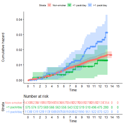
Limitations of Exponential?
Recall our Colorectal Cancer data and smoking:
suppressMessages(library(foreign))
phscrc <- read.dta("https://drive.google.com/uc?export=download&id=0B8CsRLdwqzbzSno1bFF4SUpVQWs")
crc.haz <- survfit(Surv(cayrs, crc) ~ csmok, data= phscrc, type='fleming')
suppressMessages(library(survminer))
ggsurvplot(crc.haz, conf.int = TRUE,
           risk.table = TRUE, risk.table.col = "strata",
           fun = "cumhaz", legend.labs = c("Non-smoker", "<1 pack/day", ">1 pack/day"),
          break.time.by=1)
Limitations of Exponential?
The Weibull Distribution
We use the Weibull many times as an alternative to the exponential
The weibull has
- \(h(t) = \lambda\left(\gamma t^{\gamma-1}\right)\)
- \(\Lambda(t) = \lambda t^{\gamma}\)
- \(S(t) = e^{-\lambda t^\gamma}\)
- Then
- If \(\gamma=1\) we have the exponential
- If \(\gamma>1\) the hazard increases over time.
- If \(\gamma<1\) the hazard decreases over time.
Regression
The model for weibull hazard is
\[h(t|X_1,\ldots,X_p ) = \lambda\gamma t ^{\gamma-1}\exp\left(\beta_0+\beta_1x_1+\cdots\beta_px_p\right)\]
Then
- baseline hazard is \(\lambda\gamma t ^{\gamma-1}\) and depends on \(t\)
- Covariates have a multiplicative effect on baseline hazard
- hazards for 2 covariate levels are proportional
- Can be fit in R using
survreg()
When can we do Weibull?
Weibull is not always applicable in some settings. For example
- If hazard increases of time (\(\lambda>1\)) then hazard is 0 at time \(t=0\)
- If hazard decreases of time (\(\lambda<1\)) then hazard is \(\infty\) at time \(t=0\)
Why do we use parametric models?
- If the model for \(T\) is correct that we gain power with parametric models over KM and logrank.
- If the model for \(T\) is incorrect, parametric methods will be biased and non-parametric models will not be
- It is easier to control for confounding and to detect effect modification with parametric modeling.
Parametric Regression
Exponential
For a time to event \(T\) and covariates \(X_1, \ldots , X_p\) the exponential regression model is:
\[h(t|X_1,\ldots, X_p) = \exp\left(\beta_0 + \beta_1x_1 + \cdots + \beta_px_p\right)\]
The baseline hazard function is defined as the hazard function when all covariates are 0
Exponential
\[h(t|X_1=0,\ldots, X_p=0) = \exp\left(\beta_0 \right) = h_0(t) = h_0\]
Thus we can rewrite the model as: \[h(t|X_1,\ldots, X_p) = h_0\exp\left( \beta_1x_1 + \cdots + \beta_px_p\right)\]
This suggest that covariate effects are **multiplicative* on the constant baseline hazard, \(h_0\).
Weibull
For a time to event \(T\) and covariates \(X_1, \ldots , X_p\) the Weibull regression model is:
\[h(t|X_1,\ldots, X_p) = \gamma t^{\gamma-1}\exp\left(\beta_0 + \beta_1x_1 + \cdots + \beta_px_p\right)\] with baseline hazard \[h_0(t) = \exp(\beta_0)\gamma t^{\gamma-1} = \lambda\gamma t^{\gamma-1}\] We can rewrite this as \[h(t|X_1,\ldots, X_p) = h_0(t)\exp\left(\beta_1x_1 + \cdots + \beta_px_p\right)\]
Weibull
The general Proportional Hazards Model is \[h(t|X_1,\ldots, X_p) = h_0(t)\exp\left(\beta_1x_1 + \cdots + \beta_px_p\right)\]
\[\text{or}\]
\[\log\left[h(t|X_1,\ldots, X_p)\right] = \log\left[h_0(t)\right] + \beta_1x_1 + \cdots + \beta_px_p\]
where \(h_0(t)\) is the baseline hazard function and the "intercept" is \(\log\left[h_0(t)\right]\).
Semi-Parametric Regression
- Weibull and Exponential are examples of parametric proportional hazards models, where \(h_0(t)\) is a specified function.
- In 1972, Cox generalized these types of models so that we can make inferences on the \(\beta_1, \ldots,\beta_p\) without specifying \(h_0(t)\).
- We call Cox a semi-parametric regression model
- We fit this using something called Partial Likelihood Estimation
- Once again we use an algorithm to maximize the partial likelihood.
Interpeting the Model
Let
- \(X=0\) be the control group
- \(X=1\) be the treatment group
Then
\[\begin{aligned} h(t|X=x) &= h_0(t)\exp(\beta x)\\ h(t|X=0) &= h_0(t)\\ &= \text{ baseline hazard for control group}\\ h(t|X=1) &= h_0(t)\exp(\beta)\\ &= \text{ hazard for treated group}\\ \exp(\beta) &= \dfrac{h(t|X=1)}{h(t|X=0)}\\ \end{aligned}\]
Interpeting the Model
- This means that the hazard ratio is constant over time (Proportional Hazards)
- \(\beta\) is the log hazard ratio or log-relative risk
- According to the Cox model
\[\begin{aligned} \log\left[h]h(t|X=0)\right] &= \log\left[h_0(t)\right]\\ \log\left[h]h(t|X=1)\right] &= \log\left[h_0(t)\right] + \beta\\ \end{aligned}\]
- This means the log of the hazard functions are parallel over time.
- We make no assumptions about \(h_0(t)\).
Verifying Proportional Hazards Assumption
Recall \[S(t) = \exp\left(-\Lambda(t)\right)\] with a binary \(X\) we have that
\[\begin{aligned} \Lambda_1(t) &= \Lambda_0(t)\exp(\beta)\\ S_0(t) &= \exp(\Lambda_0(t))\\ -\log(S_0(t)) &= \Lambda_0(t)\\ \log(-\log(S_0(t))) &=\log(\Lambda_0(t))\\ \end{aligned}\]
Verifying Proportional Hazards Assumption
\[ \begin{aligned} S_1(t) = exp(-\Lambda_1(t)) &= \exp\left[\Lambda_0(t)\exp(\beta)\right]\\ -\log(S_1(t)) &= \Lambda_0(t)\exp(\beta)\\ \log(-\log(S_1(t))) &= \log(\Lambda_0(t)) + \beta\\ \end{aligned} \]
Verifying Proportional Hazards Assumption
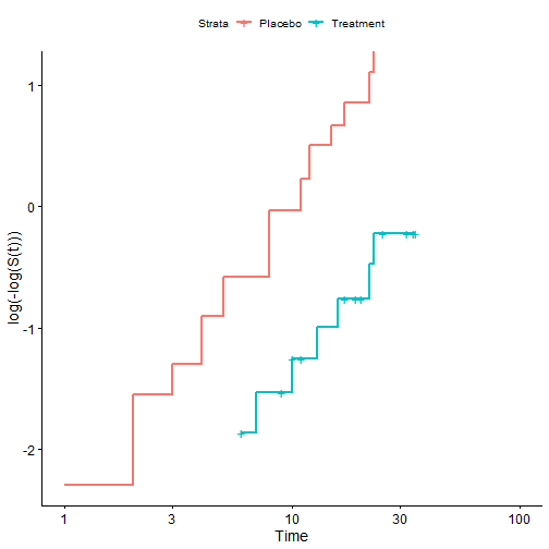
Thus we can see that under the assumption of proportional hazards
- \(\log(-\log(K-M))\) should be parallel over time.
- We typically verify this graphically.
- Recall the Leukemia study:
ggsurvplot(leukemia.surv,
      legend.labs = c("Placebo", "Treatment"),break.time.by=5,
            fun="cloglog")
Verifying Proportional Hazards Assumption
Cox PH in R
cox.leukemia <- coxph(Surv(T.all, event.all) ~ group.all , data=leuk2 )
summary(cox.leukemia)
Cox PH in R
## Call:
## coxph(formula = Surv(T.all, event.all) ~ group.all, data = leuk2)
##
##   n= 42, number of events= 30
##
##             coef exp(coef) se(coef)     z Pr(>|z|)
## group.all -1.572     0.208    0.412 -3.81  0.00014 ***
## ---
## Signif. codes:  0 '***' 0.001 '**' 0.01 '*' 0.05 '.' 0.1 ' ' 1
##
##           exp(coef) exp(-coef) lower .95 upper .95
## group.all     0.208       4.82    0.0925     0.466
##
## Concordance= 0.69  (se = 0.041 )
## Rsquare= 0.322   (max possible= 0.988 )
## Likelihood ratio test= 16.4  on 1 df,   p=0.00005
## Wald test            = 14.5  on 1 df,   p=0.0001
## Score (logrank) test = 17.2  on 1 df,   p=0.00003
This would suggest that the hazard for those in a placebo group is 4.8 times that of those in the treated group.
Cox PH in R
For another example could look at Colorectal Cancer in the PHS:
crc.cox <- coxph(Surv(cayrs, crc) ~ csmok + age , data= phscrc)
summary(crc.cox)
Then we could say that for two people with the same smoking status a one year increase in age would lead to an 8.2% increase in the hazard of colorectal cancer with a 95% CI of 6.9% to 9.6%.
Cox PH in R
## Call:
## coxph(formula = Surv(cayrs, crc) ~ csmok + age, data = phscrc)
##
##   n= 16018, number of events= 254
##    (16 observations deleted due to missingness)
##
##          coef exp(coef) se(coef)     z Pr(>|z|)
## csmok 0.31715   1.37320  0.09767  3.25   0.0012 **
## age   0.07904   1.08224  0.00628 12.58   <2e-16 ***
## ---
## Signif. codes:  0 '***' 0.001 '**' 0.01 '*' 0.05 '.' 0.1 ' ' 1
##
##       exp(coef) exp(-coef) lower .95 upper .95
## csmok      1.37      0.728      1.13      1.66
## age        1.08      0.924      1.07      1.10
##
## Concordance= 0.724  (se = 0.015 )
## Rsquare= 0.01   (max possible= 0.262 )
## Likelihood ratio test= 160  on 2 df,   p=<2e-16
## Wald test            = 163  on 2 df,   p=<2e-16
## Score (logrank) test = 177  on 2 df,   p=<2e-16
Weibull Regression
library(SurvRegCensCov)
crc.exp <- survreg(Surv(cayrs, crc) ~ csmok + age, data= phscrc, dist='weibull')
ConvertWeibull(crc.exp)
Weibull Regression
## $vars
##          Estimate         SE
## lambda 0.00000664 0.00000295
## gamma  1.30451991 0.07929445
## csmok  0.31804318 0.09766224
## age    0.07916154 0.00627915
##
## $HR
##         HR   LB   UB
## csmok 1.37 1.13 1.66
## age   1.08 1.07 1.10
##
## $ETR
##         ETR    LB    UB
## csmok 0.784 0.675 0.910
## age   0.941 0.930 0.952