
Bootstrapping
Adam J Sullivan
Assistant Professor of Biostatistics
Brown University
Resampling Methods
Resampling Methods
- Very popular tool in modern statistics.
- Involvees drawing samples from data and calculating statistics in the sample.
- Quick Example: Getting standard error and confidence intervals for non-normal data in linear regression
Resampling Methods
Why Resampling
- SO far we have been using the validation or hold-out approach to estimate the prediction error of our predictive models.
- This involves randomly dividing the available set of observations into two parts, a training set and a testing set (aka validation set).
- Our statistical model is fit on the training set, and the fitted model is used to predict the responses for the observations in the validation set.
Why Resampling
- The resulting validation set error rate (typically assessed using MSE in the case of a quantitative response) provides an estimate of the test error rate.
- The validation set approach is conceptually simple and is easy to implement. But it has two potential drawbacks:
Bootstrapping
- Bootstrapping is a widely applicable and extremely powerful statistical tool that can be used to quantify the uncertainty associated with a given estimator or statistical learning method.
- As a simple example, bootstraping can be used to estimate the standard errors of the coefficients from a linear regression fit.
- This may not seem necessary because we already achieve these through R, but bootstrapping may yield better standard errors.
Bootstrapping
- Other statistical methods are not as simple to get errors from.
- Bootstrapping can be a great way to understand variability.
What does it do?
- Basically, bootstrapping treats the data as a population.
- The we repeatedly draw independent samples to create bootstrapped datasets.
- We sample with replacement, allowing observations to be sampled more than once.
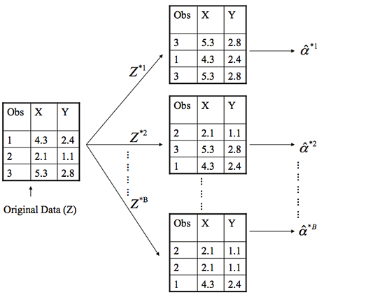
How do we do this?
- Each bootstrap data set \[Z^{*1}, Z^{*2}, \dots, Z^{*B}\] contains n observations, sampled with replacement from the original data set.
- Each bootstrap is used to compute the estimated statistic we are interested in \(\hat\alpha^*\).
Then what?
- We can then use all the bootstrapped data sets to compute the standard error of \[\hat\alpha^{*1}, \hat\alpha^{*2}, \dots, \hat\alpha^{*B}\] desired statistic as \[ SE_B(\hat\alpha) = \sqrt{\frac{1}{B-1}\sum^B_{r=1}\bigg(\hat\alpha^{*r}-\frac{1}{B}\sum^B_{r'=1}\hat\alpha^{*r'}\bigg)^2} \tag{4} \]
- \[SE_B(\hat\alpha)\] serves as an estimate of the standard error of \[\hat\alpha\] estimated from the original data set.
Example 1: Estimating the accuracy of a single statistic
- Performing a bootstrap analysis in R entails two steps:
- Create a function that computes the statistic of interest.
- Use the
bootfunction from thebootpackage to perform the boostrapping
The Data
- In this example we'll use the
ISLR::Portfoliodata set. - This data set contains the returns for two investment assets (X and Y).
The Goal
- Here, our goal is going to be minimizing the risk of investing a fixed sum of money in each asset.
- Mathematically, we can achieve this by minimizing the variance of our investment using the statistic \[ \hat\alpha = \frac{\hat\sigma^2_Y - \hat\sigma_{XY}}{\hat\sigma^2_X +\hat\sigma^2_Y-2\hat\sigma_{XY}} \tag{5} \]
- Thus, we need to create a function that will compute this test statistic:
The Function
statistic <- function(data, index) {
  x <- data$X[index]
  y <- data$Y[index]
  (var(y) - cov(x, y)) / (var(x) + var(y) - 2* cov(x, y))
}
Computing
- Now we can compute \[\hat\alpha\] for a specified subset of our portfolio data:
portfolio <- ISLR::Portfolio
statistic(portfolio, 1:100)
## [1] 0.576
How does Bootstrapping work?
-
Next, we can use
sampleto randomly select 100 observations from the range 1 to 100, with replacement. - This is equivalent to constructing a new bootstrap data set and recomputing \[\hat\alpha\] based on the new data set.
statistic(portfolio, sample(100, 100, replace = TRUE))
## [1] 0.467
What do we see?
- If you re-ran this function several times you'll see that you are getting a different output each time.
- What we want to do is run this many times, record our output each time, and then compute a valid standard error of all the outputs.
- To do this we can use
bootand supply it our original data, the function that computes the test statistic, and the number of bootstrap replicates (R).
boot() function in R
set.seed(123)
boot(portfolio, statistic, R = 1000)
boot() function in R
##
## ORDINARY NONPARAMETRIC BOOTSTRAP
##
##
## Call:
## boot(data = portfolio, statistic = statistic, R = 1000)
##
##
## Bootstrap Statistics :
##     original  bias    std. error
## t1*    0.576  0.0024      0.0875
What do we get?
- The final output shows that using the original data, \[\hat\alpha = 0.5758\], and it also provides the bootstrap estimate of our standard error \[SE(\hat\alpha) = 0.0875\].
- Once we generate the bootstrap estimates we can also view the confidence intervals with
boot.ciand plot our results:
R Code
set.seed(123)
result <- boot(portfolio, statistic, R = 1000)

boot.ci(result, type = "basic")
R Code
## BOOTSTRAP CONFIDENCE INTERVAL CALCULATIONS
## Based on 1000 bootstrap replicates
##
## CALL :
## boot.ci(boot.out = result, type = "basic")
##
## Intervals :
## Level      Basic
## 95%   ( 0.396,  0.738 )
## Calculations and Intervals on Original Scale
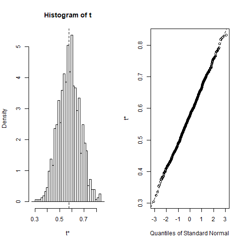
Plot of Results
Example 2: Estimating the accuracy of a linear regression model
- We can use this same concept to assess the variability of the coefficient estimates and predictions from a statistical learning method such as linear regression.
- For instance, here we'll assess the variability of the estimates for \[\beta_0\] and \[\beta_1\], the intercept and slope terms for the linear regression model that uses
horsepowerto predictmpgin ourautodata set.
The Function
- First, we create the function to compute the statistic of interest.
- We can apply this to our entire data set to get the baseline coefficients.
library(tidyverse)
auto <- as_tibble(ISLR::Auto)
statistic <- function(data, index) {
  lm.fit <- lm(mpg ~ horsepower, data = data, subset = index)
  coef(lm.fit)
}
What do we get?
statistic(auto, 1:392)
## (Intercept)  horsepower
##      39.936      -0.158
Then use boot()
set.seed(123)
boot(auto, statistic, 1000)
The Results
##
## ORDINARY NONPARAMETRIC BOOTSTRAP
##
##
## Call:
## boot(data = auto, statistic = statistic, R = 1000)
##
##
## Bootstrap Statistics :
##     original    bias    std. error
## t1*   39.936  0.029596      0.8635
## t2*   -0.158 -0.000294      0.0076
What can we conclude?
- This indicates that the bootstrap estimate for \(SE(\beta_0)\) is 0.86, and that the bootstrap estimate for \(SE(\beta_1)\) is 0.0076.
- If we compare these to the standard errors provided by the
summaryfunction we see a difference.
The summary
##
## Call:
## lm(formula = mpg ~ horsepower, data = auto)
##
## Residuals:
##     Min      1Q  Median      3Q     Max
## -13.571  -3.259  -0.344   2.763  16.924
##
## Coefficients:
##             Estimate Std. Error t value Pr(>|t|)
## (Intercept) 39.93586    0.71750    55.7   <2e-16 ***
## horsepower  -0.15784    0.00645   -24.5   <2e-16 ***
## ---
## Signif. codes:  0 '***' 0.001 '**' 0.01 '*' 0.05 '.' 0.1 ' ' 1
##
## Residual standard error: 4.91 on 390 degrees of freedom
## Multiple R-squared:  0.606,  Adjusted R-squared:  0.605
## F-statistic:  600 on 1 and 390 DF,  p-value: <2e-16
What does this mean?
- This difference suggests the standard errors provided by
summarymay be biased. - That is, certain assumptions may be violated which is causing the standard errors in the non-bootstrap approach to be different than those in the bootstrap approach.
- This may be due to the fact that this might be better modeled by a quadratic.
Quadratic Function
quad.statistic <- function(data, index) {
  lm.fit <- lm(mpg ~ poly(horsepower, 2), data = data, subset = index)
  coef(lm.fit)
}
Boot it
set.seed(1)
boot(auto, quad.statistic, 1000)
Boot it
##
## ORDINARY NONPARAMETRIC BOOTSTRAP
##
##
## Call:
## boot(data = auto, statistic = quad.statistic, R = 1000)
##
##
## Bootstrap Statistics :
##     original  bias    std. error
## t1*     23.4 0.00394       0.226
## t2*   -120.1 0.11731       3.701
## t3*     44.1 0.04745       4.329
What do we get?
- Now if we compare the standard errors between the bootstrap approach and the non-bootstrap approach we see the standard errors align more closely.
- This better correspondence between the bootstrap estimates and the standard estimates suggest a better model fit.
- Thus, bootstrapping provides an additional method for assessing the adequacy of our model's fit.
Summary in R
##
## Call:
## lm(formula = mpg ~ poly(horsepower, 2), data = auto)
##
## Residuals:
##     Min      1Q  Median      3Q     Max
## -14.714  -2.594  -0.086   2.287  15.896
##
## Coefficients:
##                      Estimate Std. Error t value Pr(>|t|)
## (Intercept)            23.446      0.221   106.1   <2e-16 ***
## poly(horsepower, 2)1 -120.138      4.374   -27.5   <2e-16 ***
## poly(horsepower, 2)2   44.090      4.374    10.1   <2e-16 ***
## ---
## Signif. codes:  0 '***' 0.001 '**' 0.01 '*' 0.05 '.' 0.1 ' ' 1
##
## Residual standard error: 4.37 on 389 degrees of freedom
## Multiple R-squared:  0.688,  Adjusted R-squared:  0.686
## F-statistic:  428 on 2 and 389 DF,  p-value: <2e-16